A street design index from streetspace allocation metrics
How can pavement and carriageway widths explain street design?
r
streetspace
sf
Author
Nicolas Palominos
Published
May, 2022
Streetspace allocation
The amount of space designated for footways and carriageways is a crucial street design parameter that can affect the streets’ environmental quality. It could be expected that streets with higher pedestrian activity would have wider pavements. To a certain extent this is confirmed by the greater association that exists between central streets and streets with wider pavements in London1. Provided the width of streets is dictated by land ownership structure which are difficult to transform, the relationship between footway and carriageway street width is a critical parameter for streetspace reallocation interventions.
This exercise examines the streetspace allocation data set published for London 2 by creating a streetspace index that quantifies footway/carriageway relationships
The streetspace allocation dataset for London
After downloading and before reading the data the following packages are loaded to run the code.
Then we can read the data (earlier the dataset was converted to RDS to reduce its size)
Code
sa <-readRDS("streetspace_dataset.rds")# read wards data# dir.create("./data_raw")target.file <-"./data_raw/wards.zip"download.file(url ="https://data.london.gov.uk/download/statistical-gis-boundary-files-london/08d31995-dd27-423c-a987-57fe8e952990/London-wards-2018.zip", destfile = target.file)unzip(target.file, overwrite =TRUE, exdir ="./data_raw/")# file.remove(target.file) # Delete the zip file# Read the unzipped filelw <-st_read("./data_raw/London-wards-2018_ESRI/London_Ward.shp", quiet =TRUE)
Creating the streetspace index
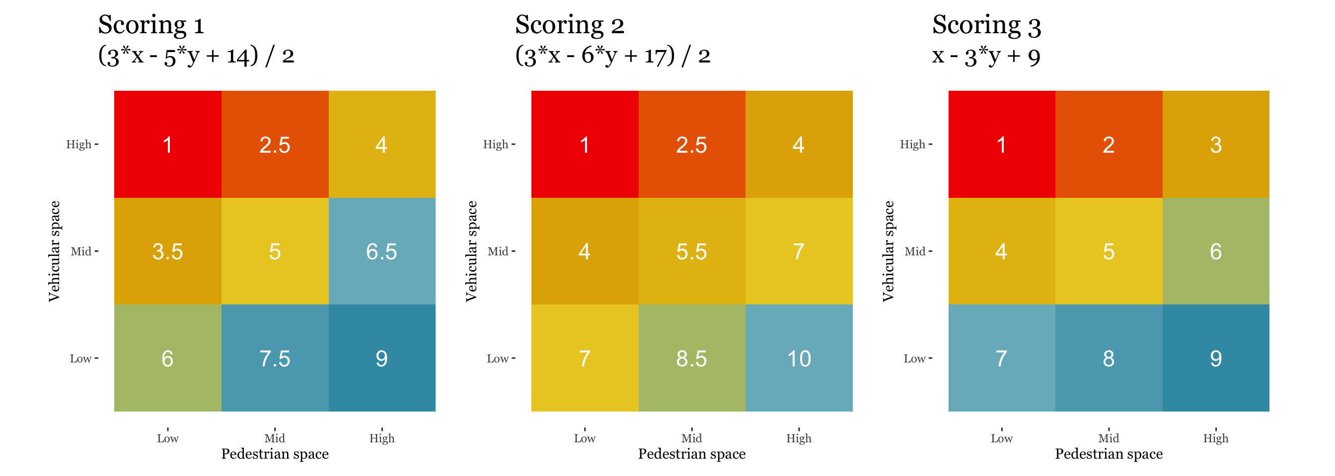
The streetspace index is calculated taking the Link and Place framework as a reference 3. A 3x3 matrix is created from 3 classes of footway and carriageways (low, mid and high widths). The matrix describes a double slope surface to which all values (footway and carriageway widths) are fitted.
An approximate score from 1-9 is assigned according streetspace allocation metrics and their relationship. I tested different plane functions (different scores) but chose Index 3 which I believe most closely approximates to the negative/positive impacts of street design in the environmental quality of streets. For example, a street with wide footway (high pedestrian space) and narrow carriageway (low vehicular space) scores 9. While a score of 1 is assigned to streets at the opposite corner of the matrix (low pedestrian space and high vehicular space). Similarly, a street with low-low space scores (7) higher than a street with high-high space (3). This assumes that the negative impact of wide carriageways (despite the presence of wide footways) is higher than the negative impact of narrow pavements (despite the presence of narrow carriageways). Overall, a general rule for this scoring matrix is that being the footway equal streets with wider carriageways have lower scores and being the carriageway equal streets with wider footways have higher scores.
Streetspace allocation scoring matrices that were tested
After selecting the scoring approach (and function: x - 3*y + 9), we can calculate the streetspace index (S-Index). This takes all footways (x) and carriageways (y) widths, apply the plane function and transform the results to a scale of 1-100
Code
sa %>%mutate(sco3 = foW -3*caW +9,# min-max normalisation * 100S_Index = ((sco3 -min(sco3)) / (max(sco3) -min(sco3))*100)) -> sai
How does the index work? The interactive plot for a sample of 10,000 streets shows the final index after applying the scoring function to the street’s footways and carriagways widths. It can be seen that the streetspace index (S-Index - scoring 3) performs better when looking at streets with the same ratio (e.g. those following the direction of the grey line). This reveals that unlike the other indices, there is a clear differentiation between streets with high-high and low-low streetspace metrics. This also applies to the extra index labelled as Diff, that take the subtraction of Footway - Carriageway widths, which won’t differentiate between streets with the same ratio.
Mapping the S-Index
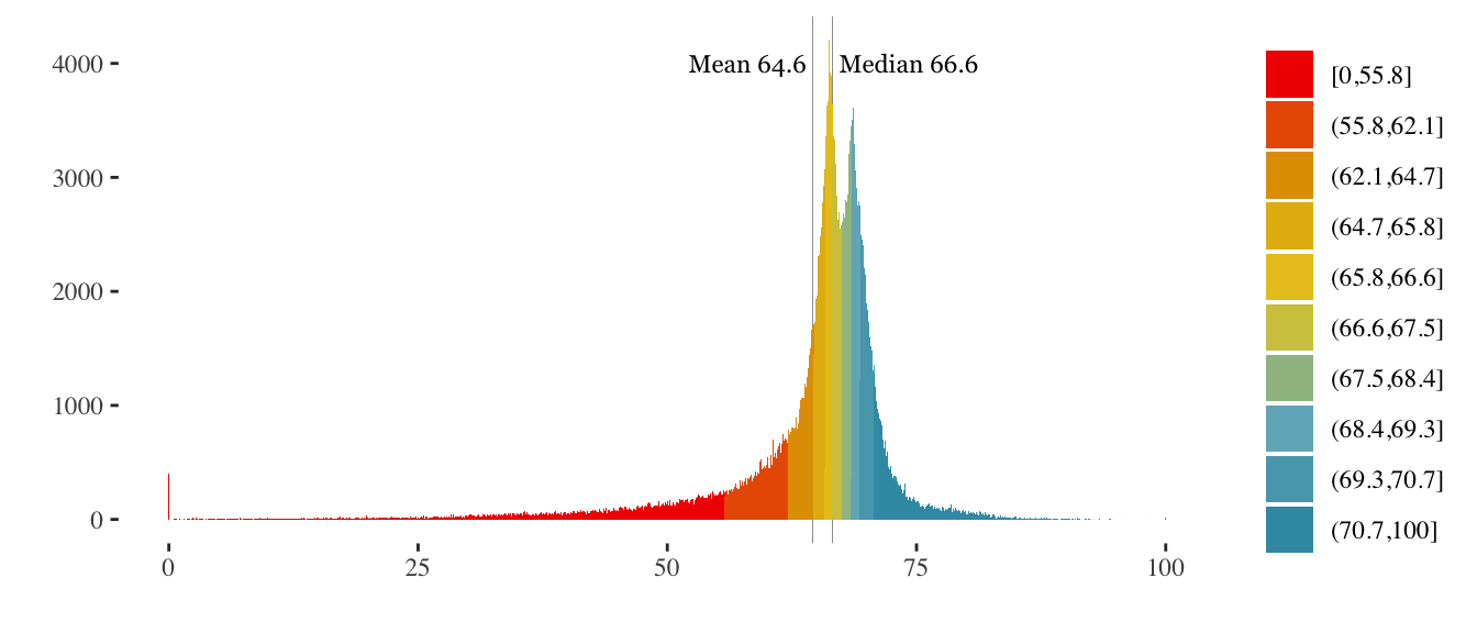
Before mapping the S-Index it is useful to look at the distribution of values, which is this case is near normal.
Code
sai %>%# make 10 groups with equal number of observationsmutate(cut =cut_number(S_Index, n =10),avg =mean(S_Index),median =median(S_Index)) %>%ggplot() +# meanannotate("text", x=mean(sai$S_Index), y=4000, label=paste("Mean", round(mean(sai$S_Index),1), sep =" "), family ="Georgia", size =3, hjust =1.05) +geom_vline(aes(xintercept =mean(S_Index)), colour="gray55", size=.15) +# medianannotate("text", x=median(sai$S_Index), y=4000, label=paste("Median", round(median(sai$S_Index),1), sep =" "), family ="Georgia", size =3, hjust =-0.05) +geom_vline(aes(xintercept =median(S_Index)), colour="gray55", size=.15) +geom_histogram(aes(S_Index, fill = cut), binwidth =0.1) +theme_tufte() +scale_fill_manual(values =colorRampPalette(mycols)(10), name ="") +labs(y ="", x="")
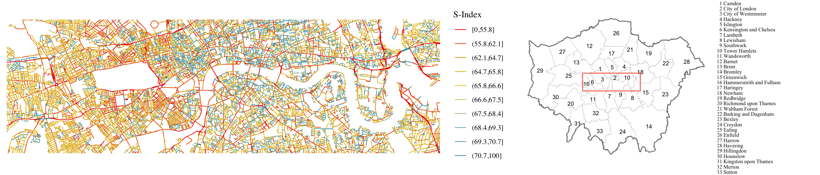
Plotting a section of London with 10 classes of the S-Index shows an interesting pattern. Main thoroughfares can be identified in the lower tiers coloured in red (potentially with higher vehicular traffic) while it is possible to identify a cluster of ‘blue’ streets in the West End area which corresponds with higher street level pedestrian activity.
Code
sai %>%mutate(cut =cut_number(S_Index, n =10)) %>%ggplot() +geom_sf(aes(col = cut), size =0.4, show.legend ="line") +scale_colour_manual(values =colorRampPalette(mycols)(10), name ="S-Index") +theme_tufte() +theme(axis.title =element_blank(),axis.text =element_blank(),axis.ticks =element_blank()) +coord_sf(expand =FALSE, xlim =c(521665.5110, 540778.3620), ylim =c(176883.0072,182798.4996), datum =27700) -> pslgrid.arrange(psl, plsec, lbnl, widths =c(5,2,1))
S-Index for a section of London
Profiling London boroughs with the S-Index
The S-Index can be summarised by Borough to compare their performance and visualise where there is opportunity for intervention. The scoring matrix in Section 0.3 shows how the reallocation of streetspace following a bottom-left direction of the matrix (low-high to high-low) will improve the S-Index. The table below shows a summary of the S-Index and street metrics by Borough. It doesn’t appear surprising that Westminster (City of Westminster) is the worst performing not only due to the large number of mayor roads crossing through the borough but also probably because of their well-known car-oriented policies.
See Jones, P., Boujenko, N. and Marshall, S., 2007. Link & Place-A guide to street planning and design↩︎
Citation
BibTeX citation:
@online{palominos2022,
  author = {Nicolas Palominos},
  title = {A Street Design Index from Streetspace Allocation Metrics},
  date = {2022-05},
  url = {https://nicolaspalominos.netlify.app/posts/streetspace-index/},
  langid = {en}
}